SNAM Pipeline Network — Redait Tsegaye Legesse

Overview

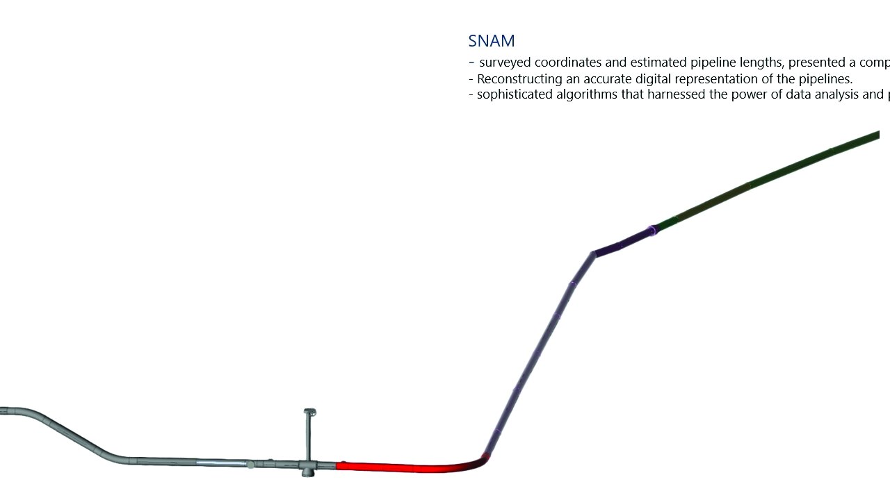
SNAM operates one of Europe’s largest natural gas transmission networks, with pipelines running across the entire Italian territory. The project required creating a complete BIM model of the existing pipeline infrastructure — not from drawings, but from raw survey data: sequences of XYZ coordinates, estimated segment lengths, and component type designations.

Italy map — SNAM national pipeline network extent — SNAM operates across the full Italian national territory

SNAM pipeline BIM model in Revit showing reconstructed pipeline geometry — Reconstructed pipeline segment in Revit — geometry generated algorithmically from coordinate data

The Problem: Data Is Not a Model

Survey data for pipeline infrastructure is rarely clean. Coordinate sets require interpretation: which points define a straight segment and which mark a bend? What type of elbow was used at a given turn — a standard curve or a barrier fitting? Where do human data-entry errors produce coordinates that break the pipeline geometry?

Manual modeling at this scale was not feasible. The solution had to be algorithmic.

The Algorithm: Elbow Type Logic

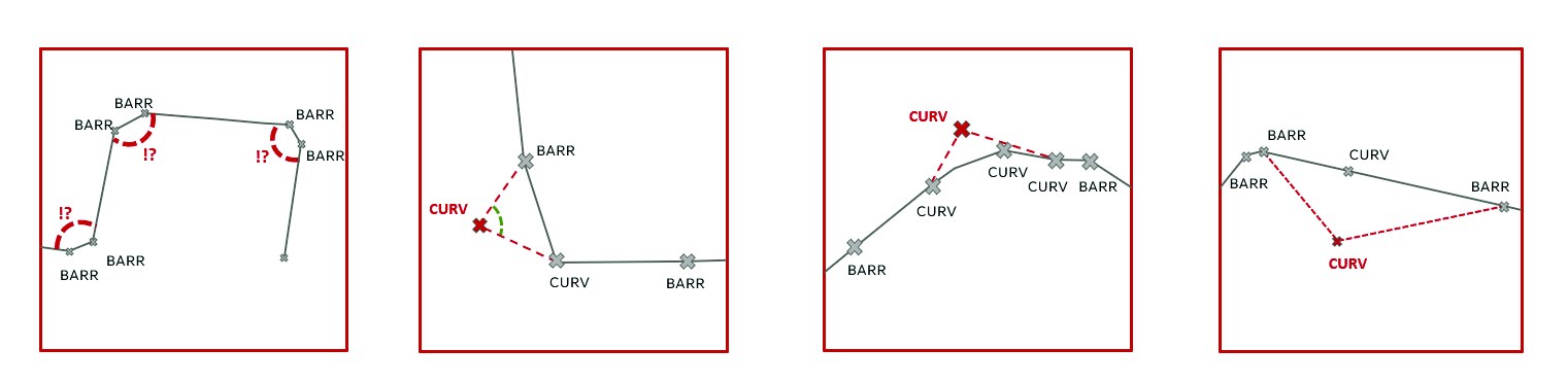
The core challenge was teaching the script to identify elbow types from the angular relationships between consecutive pipeline segments. Each junction could be one of several fitting types — CURV (curved elbow) or BARR (barrier fitting) — and the correct identification mattered for both geometry and specifications.

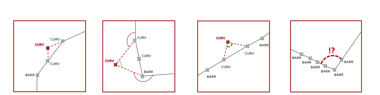
Algorithm decision diagram showing elbow type identification across four pipeline scenarios — Algorithm logic — four scenarios for elbow type identification from coordinate geometry. The script reads the angle and point configuration at each junction to determine the correct fitting type.

Real survey data produces situations that fall outside the clean scenarios: multiple BARR points clustered at a junction, CURV markers without a clear apex, ambiguous configurations flagged with !? for manual review. The algorithm was designed to handle the predictable cases automatically and surface the uncertain ones rather than making silent errors.

Extended elbow logic diagram showing ambiguous and complex multi-fitting junction scenarios — Edge cases — complex junction configurations where the algorithm flags ambiguity (!?) for human review rather than guessing. Designing for failure modes was as important as designing for the standard cases.

Result

The Grasshopper scripts processed coordinate datasets and produced fully connected pipeline geometry in Revit — with component types placed at each junction, segment lengths calculated, and all data linked to the BIM element parameters. Sections of the national network that would have taken weeks of manual modeling were reconstructed in a fraction of the time.

The more significant outcome was methodological: a reusable workflow that could be applied to additional network sections as the project expanded, with the algorithm’s behavior documented and the edge-case handling transparent.